More signal, less uncertainty
Read panel 1 from left to right: both curves descend. A cleaner observation cannot increase the optimal prediction error.
\(\gamma_2\geq\gamma_1\;\Rightarrow\;m_S(\gamma_2)\leq m_S(\gamma_1)\).
When does diffusion generate each feature?
Denoising losses reveal its implicit generation order.
1 Westlake University 2 Zhejiang University 3 Australian National University
01 · An autoregressive view of diffusion
Autoregression and diffusion make generation tractable through smaller prediction tasks: one predicts successive sequence elements, the other progressively removes noise. Inspired by Sander Dieleman’s blog, we ask what implicit generation order diffusion follows.
In pixel space, diffusion can be viewed as approximate spectral autoregression: low frequencies emerge before high frequencies. This account does not directly extend to learned latent spaces, now standard in image generation. Their markedly different convergence speeds make understanding what happens in each representation essential.
Across arbitrary representations, which features are generated at each SNR? We quantify how information about a feature—class, mask, or Canny edges—is distributed along diffusion, then study the order in which multiple features emerge.
02 · Feature information density
Let \(X_\gamma\coloneqq\sqrt{\gamma}X+N\) be the noisy observation at SNR \(\gamma\), with independent standard Gaussian noise. Mutual information \(I(Y;X_\gamma)\) measures how much it contains about feature \(Y\). We define feature information density as its rate of change along log-SNR; I-MMSE connects this rate to optimal denoising losses:
Here \(m_S(\gamma)\) is the minimum x-prediction loss (MMSE) given condition \(S\). Below, \(Y\) is the MNIST digit class. The unconditional denoiser predicts the clean image from the noisy image alone; the class-conditional denoiser also receives its class label. Their optimal losses are \(m_{\varnothing}\) and \(m_Y\), respectively.
\(m_{\varnothing},\;m_Y\)
━ Unconditional
━ Class-conditional
Both curves fall with SNR; their shaded separation is the conditioning gain.
\(\Delta_Y\coloneqq m_{\varnothing}-m_Y\)
Subtract the two optimal losses.
\(D_Y^{(\ln\gamma)}=\frac{\gamma}{2}\Delta_Y\)
The rate of class information gain along log-SNR. Its peak locates the fastest emergence.
\(\begin{aligned}&\int_{-\infty}^{\ln\gamma}D_Y^{(\ln\gamma)}(u)\,du\\&\qquad=I(Y;X_\gamma)\end{aligned}\)
Integrate feature information density over ln SNR up to the selected SNR.
Drag the slider or click a curve to explore. Images show one digit; curves average the full test set. Measured losses estimate MMSE.
Read panel 1 from left to right: both curves descend. A cleaner observation cannot increase the optimal prediction error.
\(\gamma_2\geq\gamma_1\;\Rightarrow\;m_S(\gamma_2)\leq m_S(\gamma_1)\).
At panel 1’s cursor, teal lies below gray. Their shaded separation is the gap in panel 2. Extra conditions cannot increase optimal loss: a denoiser can ignore them.
\(m_{S,Y}(\gamma)\leq m_S(\gamma)\). In particular, feature information density is nonnegative: \(D_Y^{(\ln\gamma)}\geq0\).
For the Gaussian channel \(X_\gamma\coloneqq\sqrt{\gamma}X+N\) with independent standard Gaussian noise \(N\), MMSE is the minimum clean-data prediction loss, attained by the conditional mean:
Other diffusion targets require conversion. For Gaussian flow matching, \(X_t\coloneqq(1-t)N+tX\), \(\gamma\coloneqq(t/(1-t))^2\), and MMSE equals the minimum velocity loss multiplied by \((1-t)^2\).
Trained-model losses approximate these optima; measured curves need not satisfy the exact inequalities. The raw signed MNIST integral is 2.626 nats versus label entropy 2.301 nats (14.1% error). The theoretical cumulative information integrates from log-SNR minus infinity; the numerical estimate uses the displayed finite SNR range. Class generation progress is normalized over that range. Normalization does not remove estimation error. The images are fixed-noise denoising probes, not a reverse-sampling trajectory, and the percentage measures population information rather than one image’s confidence.
§3.1–3.4 · MMSE, information density, and estimation · Run the notebook
03 · Chained information decomposition
Frequency bands share information, so measuring each independently can obscure their generation order. Our chained decomposition measures what each band adds beyond those already given. These increments sum to the joint feature information density:
Here \(m_k\) is the optimal denoising loss given the first \(k\) frequency bands; \(m_0\) is unconditional.
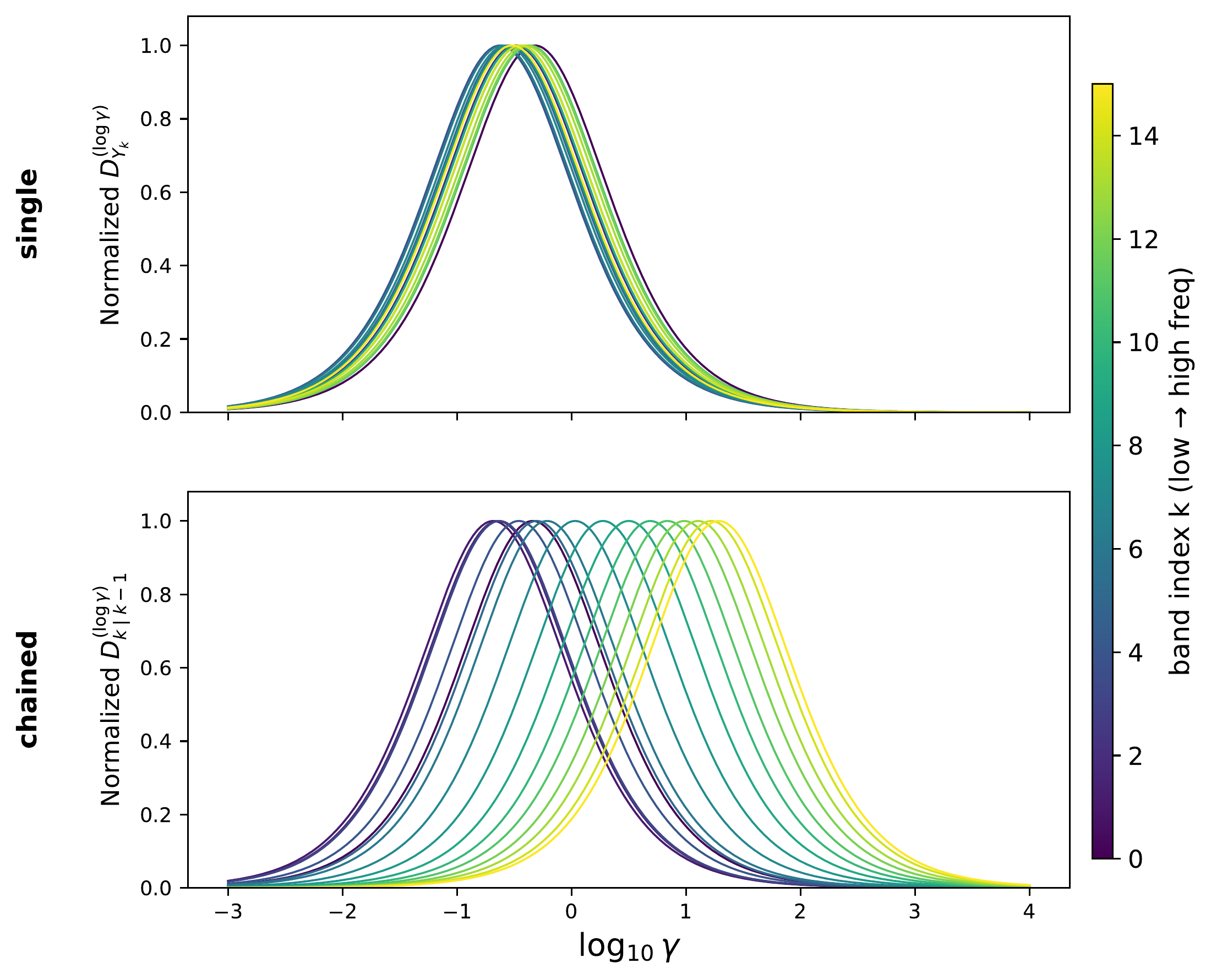
§4 · Chained information decomposition · §5.1 · Spectral autoregression
04 · Representations change generation order
We extend the analysis beyond frequency to a more complex visual hierarchy: class → mask → Canny. Conditioning in this order, we compare when each feature’s incremental information appears across pixels and three latent spaces.
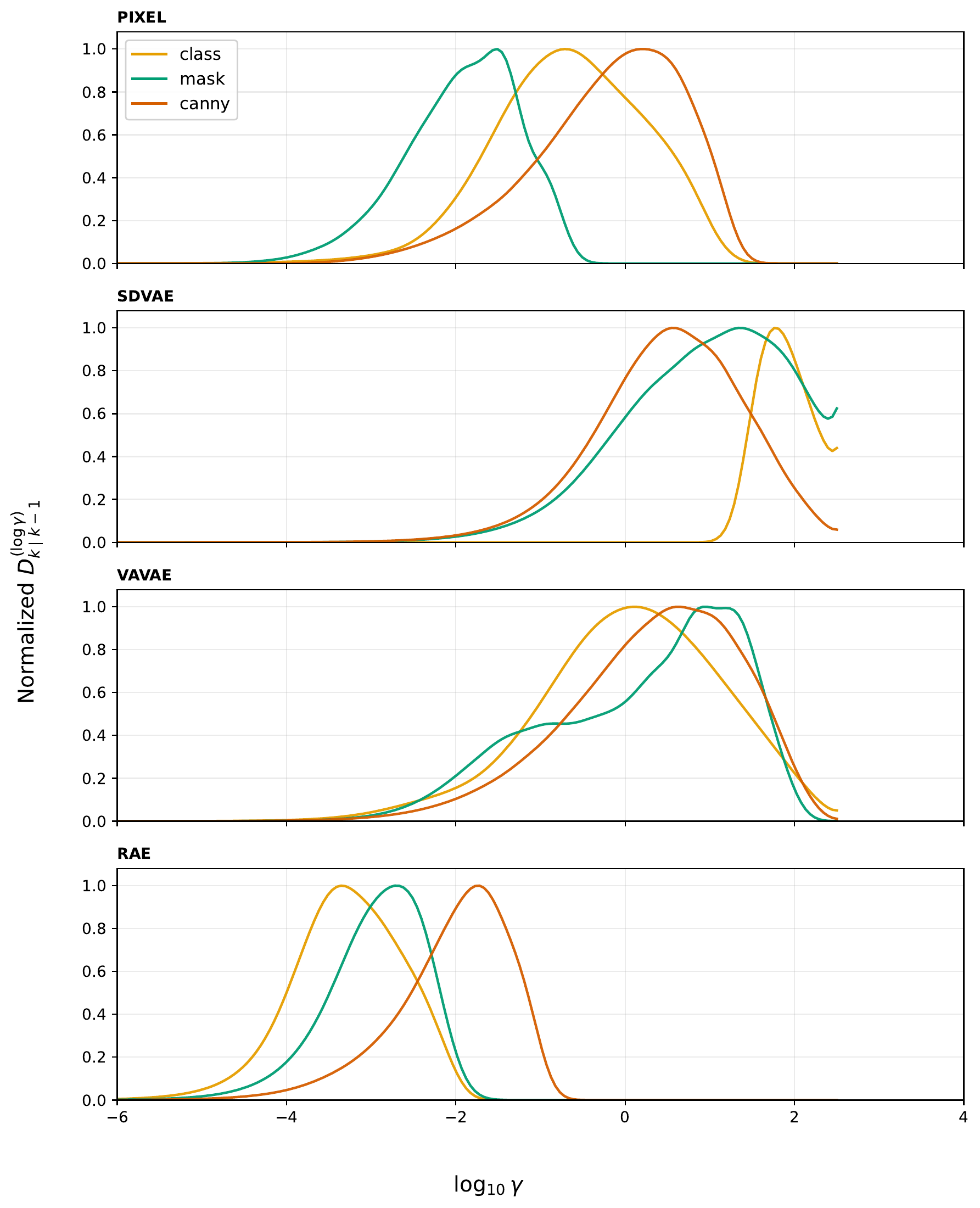
Mask information peaks before class information.
Class information peaks after shape and local boundaries.
Class leads, but object shape and local boundaries still overlap.
Only RAE clearly separates the peaks in class → mask → Canny order, from semantic identity to local detail.
AO-GPT finds that left-to-right language modeling converges much faster than a fixed random order, attributing this advantage to language’s sequential structure.
Our observation is suggestive: RAE generates from semantic identity to local detail and converges faster than pixels, SDVAE, and VAVAE. We conjecture that images favor generation from abstract to concrete.
How can we discover the best generation order for each modality? Could those orders guide the next generation of generative models?
Controlled convergence comparison · §5.2.2 · Representation diagnostics · §6.1 · Generation order